As common as it is, the central limit theorem makes a critical assumption that is easy to gloss over: the distribution you’re sampling from must have finite variance 1. The reason I think it’s easy to gloss over is that one is rarely shown examples of distributions with infinite variance.
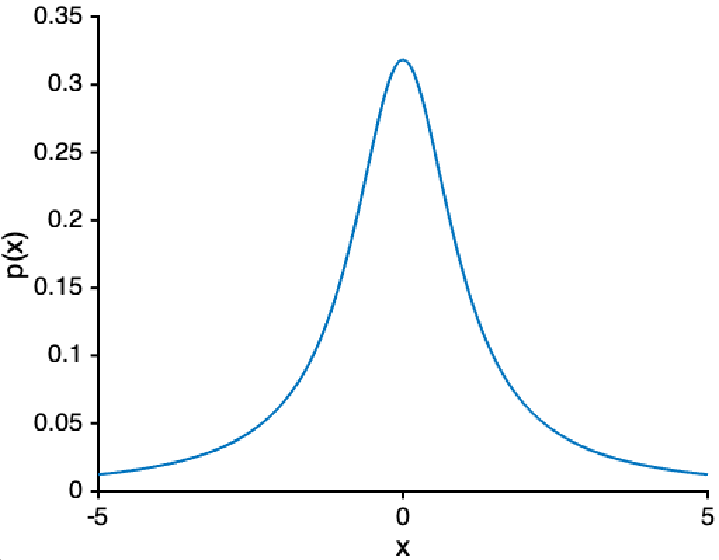
It turns out that the Cauchy distribution, Student’s t, Pareto distribution (aka the “power-law distribution”), and more all have infinite (or undefined) variance. Look at the Cauchy distribution below:

It’s not at all obvious by eye that the variance of the distribution above is infinite 2. When a distribution’s variance is infinite/undefined, it’s typically because there is always some small-but-not-negligible chance that you’ll sample an extraordinarily large value. This is what people mean when they say a distribution has “fat tails.” One weird property of having fat tails is that you may be no better off estimating the distribution’s mean using the mean of \(N = 100,000\) samples than with a sample of \(N = 1\). And that is certainly the opposite of what the central limit theorem claims.
So let’s say we have \(N\) independent samples \(X_1, \ldots, X_N\) from some distribution \(P\). If the variance of \(P\) is infinite, the central limit theorem does not apply. So what can we do? Well, it turns out there is a generalization of the central limit theorem that does not require the variance of \(P\) to be finite. In this case, the sum \(\sum_{i=1}^N X_i\) converges in distribution to a symmetric alpha-stable distribution with parameter α, aka a stable distribution 3. The value of α is based on how fast the tails decay. When α ≥ 2, this is equivalent to a Gaussian distribution—in other words, we get the central limit theorem. But when α < 2, we get a different distribution entirely. For example, α = 1 is a Cauchy distribution. This means that taking sums of \(N\) samples from a Cauchy distribution (shown above) will not eventually become a Gaussian…it will remain Cauchy!
Notes
-
While it may be common in practice to assume your data comes from a distribution with finite variance, this is not always the case. For example, both stock market fluctuations and extreme weather events may have extreme events that occur more often than predicted by a Gaussian distribution. In these cases, when your variance is unbounded, the central limit theorem does not apply. ↩
-
In fact, the Cauchy distribution doesn’t have a variance or a mean! ↩
-
The family of “stable” distributions are so-called because if \(X_1, \ldots, X_N\) are samples from a stable distribution with some parameters, then the sum \(\sum_{i=1}^N X_i\) also has a stable distribution. This means you can think of a stable distribution as a sort of “attractor” for sums of random variables. ↩