High-dimensional data doesn't always look how you think it will

There are a number of ways of visualizing low-dimensional data. When we have data in two-dimensions, for example, we can just make a plot. Unfortunately, the intuitions we get from visualizing 2d and 3d data can often mislead us when we try to think about data with more dimensions. For example:

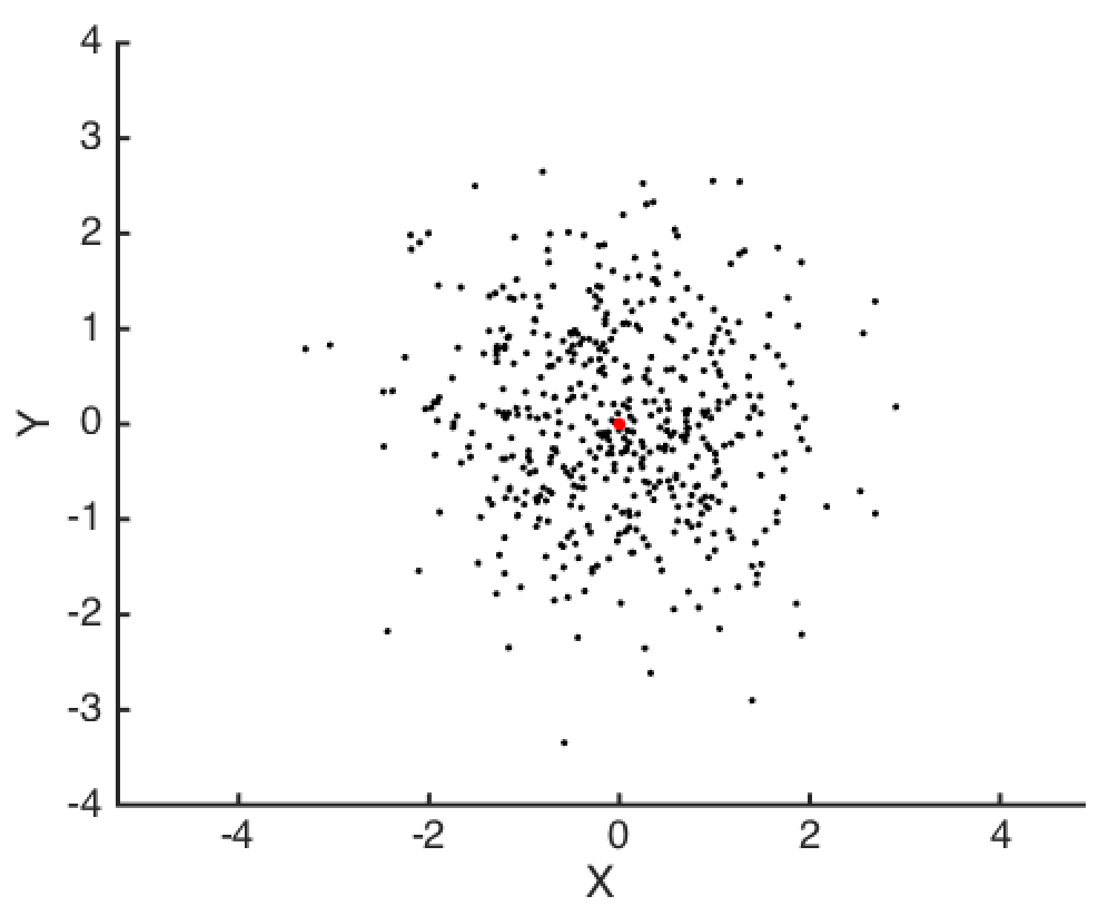
Above, I’ve plotted \(N=500\) random draws from two independent standard normals: \(X, Y \sim N(0,1)\). One natural question to ask next might be “How far are these data points from the origin?”

The distance of each point \((X_i, Y_i)\) from the origin is easy enough to compute: It’s \(V_i = \sqrt{X_i^2 + Y_i^2}\). But \(X\) and \(Y\) are random variables, and so it turns out that we know \(V\) will follow a chi distribution with 2 degrees of freedom: \(V \sim \chi(2)\).

By looking at a histogram for \(V_i\), we can see that most of our data has a distance of 1 from the origin. We can actually know this without making a plot, though, because we know the mode of a \(\chi(k)\) distribution is \(\sqrt{k-1}\), where in this case we have \(k=2\). Also, using the CDF of \(\chi(k)\), we know that on average, \(39\)% of the data will have a distance of less than 1 to the origin¹.

Now let’s see what happens if we have 3d data. Below we have \(N=500\) random draws for \(X, Y, Z \sim N(0,1)\).

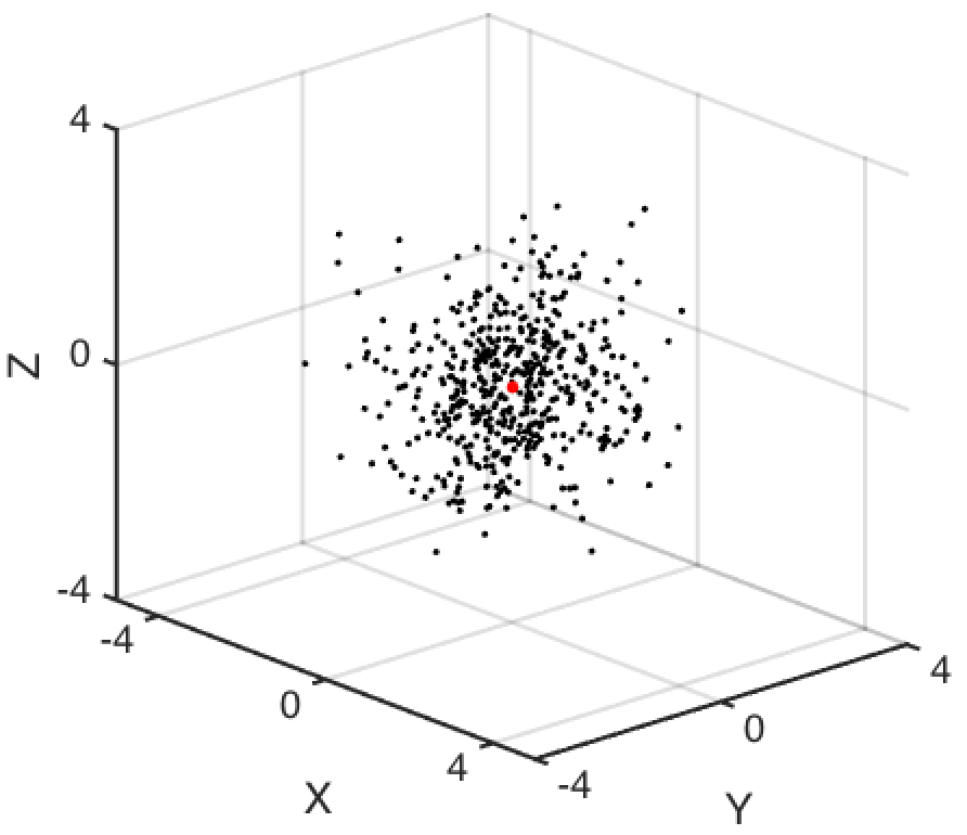
As before, we’d like to know how far these data points are from the origin. This distance is now \(V_i = \sqrt{X_i + Y_i + Z_i}\), which is a chi random variable with 3 degrees of freedom. Below, you can see that now most of our data has a distance of \(\sqrt{2}\) from the origin. That’s because the mode of a \(\chi(3)\) distribution is \(\sqrt{3-1} = \sqrt{2}\).

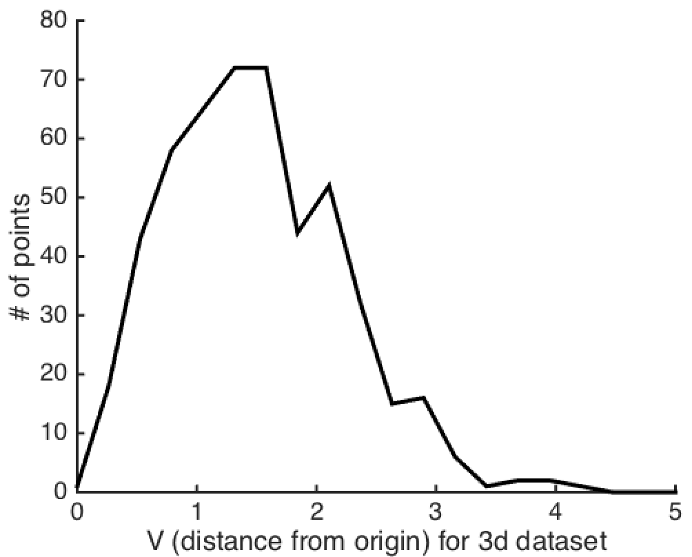
Finally, let’s suppose our data has \(k\) dimensions, where \(k\) is something larger than 3. Imagine for example that \(k=20\). The problem is that now we don’t have a way of visualizing this data all at once, but we still might want to know how far our data are from the origin. Following the logic above, the distribution of the distance of our points from the origin will be \(\chi(k)\), and so the mode will be \(\sqrt{k-1}\).

But something weird happens in high dimensions that you might not expect just from thinking about the examples when \(k=2\) and \(k=3\): As you add more and more dimensions, your data will get further and further away from the origin. In fact, as you add more and more dimensions, there becomes basically no chance that any of your data will be a distance less than 1 from the origin²:

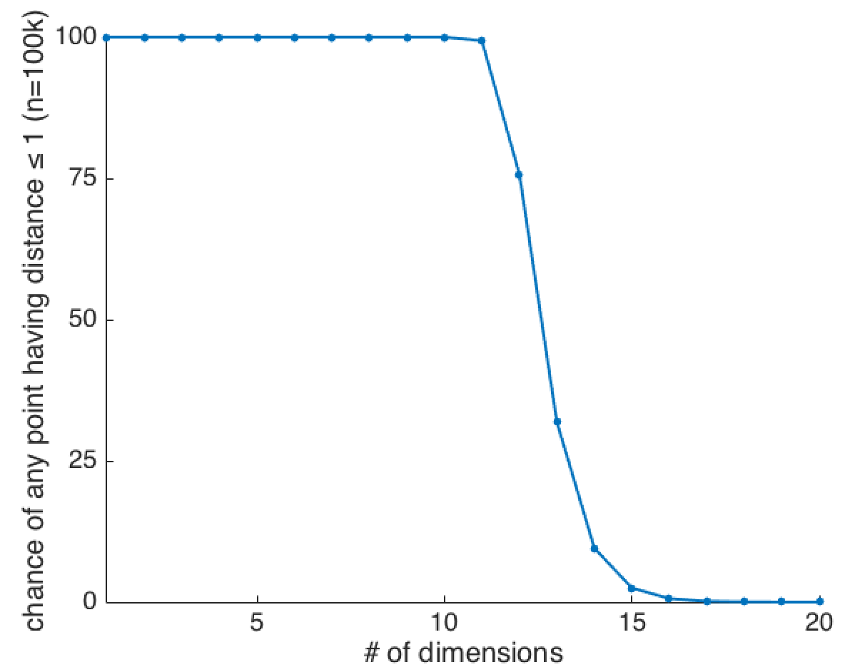
This is weird: As the number of dimensions increases, the data get essentially further and further from the origin. When \(k=20\), even if you sample \(100,000\) points, the probability of there being any data with distance less than 1 is about \(0.0017\)%. What this means is that when \(k=20\), we’re basically guaranteed that we could draw a 20-dimensional ball with radius 1 that wouldn’t have any data inside of it³. It’s almost as if a low-dimensional picture of what’s going on in high-d looks more like this, conceptually:

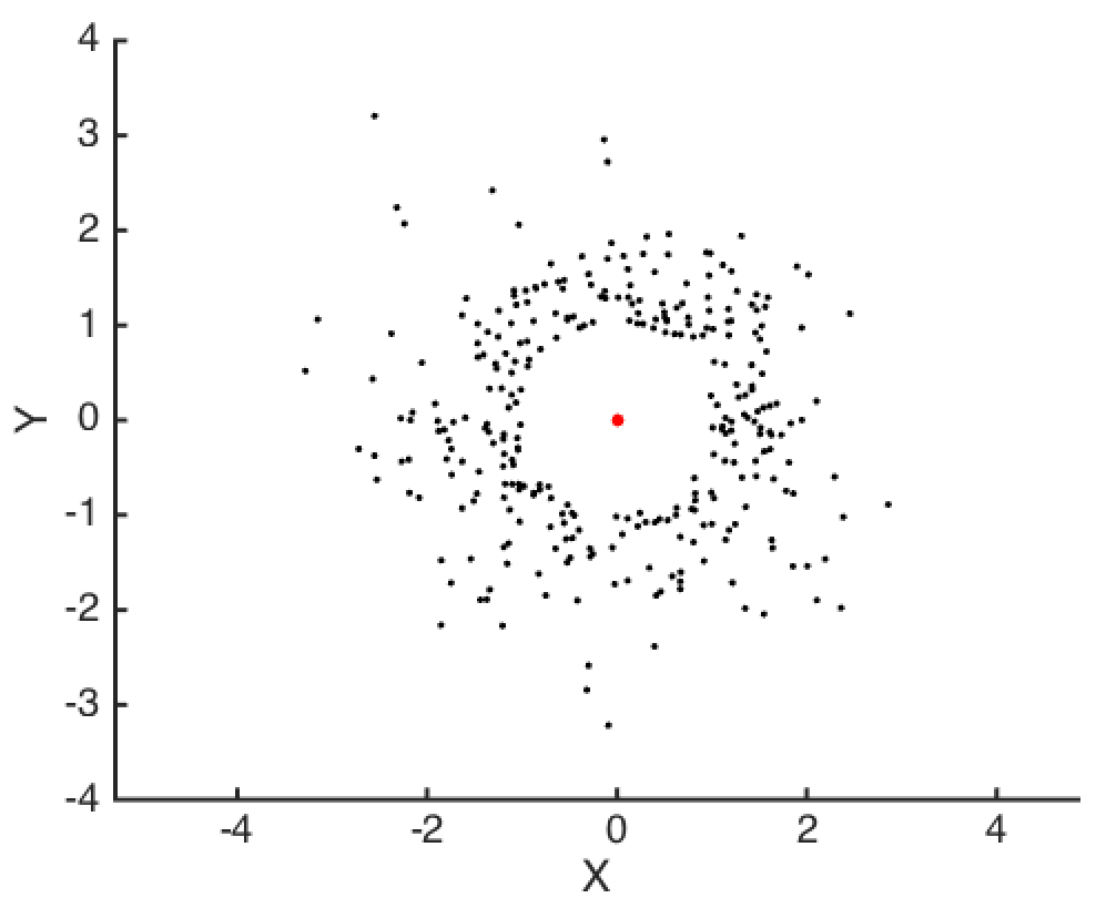
This makes perfect sense if you were to think about things probabilistically⁴. It’s only when we think about the outcome graphically that we find our intuitions about 2d and 3d data lead us astray.

---

Notes